A. Vicente Arévalo
  • About
  • Work
  • CV
  • GitHub

Andrés Vicente Arévalo

Astrophysicist and ML researcher. I turn noisy measurements into physical answers, and make the slow part fast: inverse problems, graph neural networks and HPC.
AstrophysicistInverse problemsGraph neural networksHPC

I turn noisy measurements into physical answers — and make the slow part fast.

Solar physicist at the Leibniz Institute for Solar Physics. I build inversion codes that recover the Sun's magnetic field from polarised light, and graph-neural-network surrogates that make the radiative transfer behind them 10³ to 10⁶ times faster.

Now looking to bring that toolkit — inverse problems, 3D modelling, PyTorch and supercomputer-scale data — to research-scientist, data-science and machine-learning roles.
View CV Research & code [email protected]
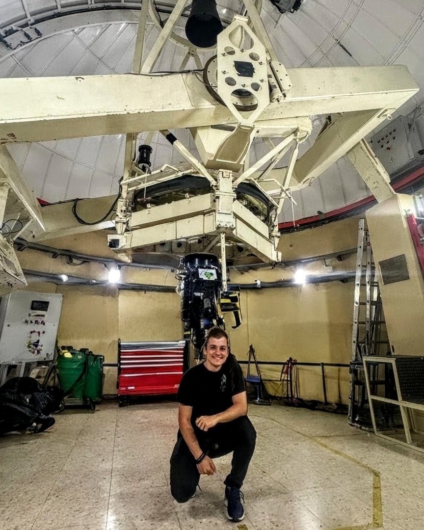
Andrés Vicente Arévalo kneeling beneath a telescope inside an observatory dome
Selected figures

Three results, one visual each

All three are live: rotate the prominence, pick any pixel of the sunspot, turn the graph.
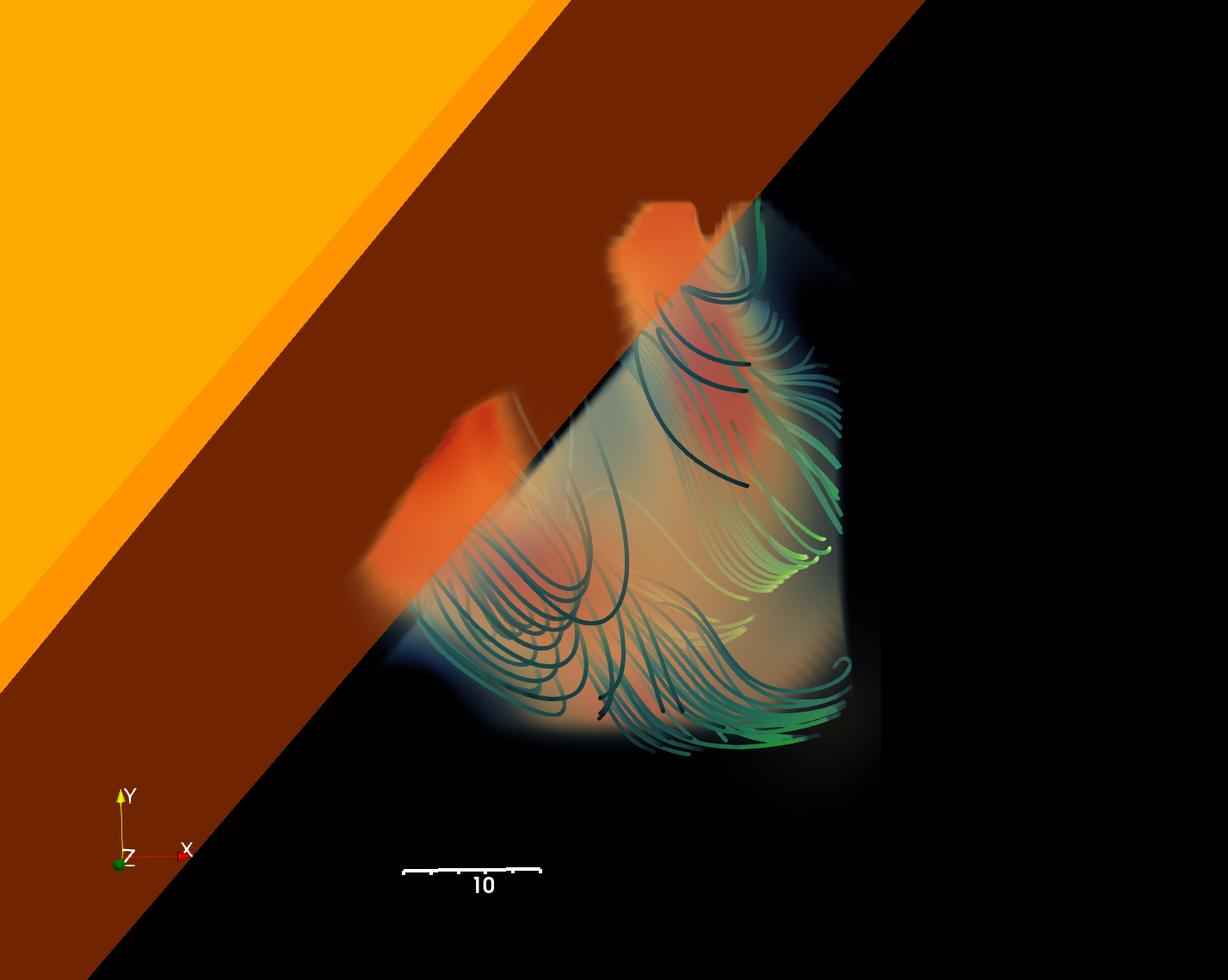
Volume rendering of the reconstructed prominence: two dense orange feet joined by fainter plasma, threaded by green magnetic-field lines, beside the solar limb.
3D prominence, He I 10830 Å
Two dense feet bridged by rarefied plasma; depth along the line of sight recovered from radiative transfer alone. Orange is the ortho-helium density from the POLARIS inversion, green the field lines of the inferred magnetic field. In preparation (ApJ Letters).
The reconstruction itself, not a video: rotate it, zoom in, switch the plasma, field lines and Sun on and off.
Observed intensity at the Fe I 630.2 nm continuum: the dark umbra, the filamentary penumbra around it, and granulation.Observed intensity, Fe I 630.2 nm continuum, 0.15 to 1.07 of the quiet Sun
Temperature 1,236 km up (mean log τ −5) over the sunspot: a hot patch in the umbra, the umbral flash, inside a cooler ring, with radial fibrils around it.Temperature at z = 1,236 km (mean log τ −5), 4.7 to 7.3 kK
Sunspot: photosphere → chromosphere
The FIRTEZ inversion of a sunspot observed with CRISP at the Swedish Solar Telescope in four lines (Fe I, Na I D1, Ca II and Mg I b2), with non-LTE and magnetohydrostatic equilibrium, on a geometrical height scale. Pick a pixel on either map for its observed and fitted Stokes profiles and its temperature, velocity and magnetic field against optical depth; the field is in the observer’s frame, z along the line of sight. The first pixel sits in an umbral flash: the Ca II core is in emission and the chromosphere above it is hot. A&A 2026.
The web version of the GUI I check inversions with. Dots are the wavelengths CRISP observed; the fit spans the inversion’s whole grid; Stokes parameters are in units of the quiet-Sun continuum. The 40 GB of data are averaged over 6 × 6 pixels and stored as principal components: 3.2 MB to start; Q, U, V and the initial guess load when picked.
Context nodesTarget columndrag to rotate · hover a node
10⁶×faster than the numerical solver, in 3D
speed-up over the numerical solver (log scale)
Solver
1×
GNN · 1D
10³×
GNN · 3D
10⁶×

1D on one CPU; 3D on one H100 GPU against a CPU cluster.

GNN surrogate vs. classical non-LTE
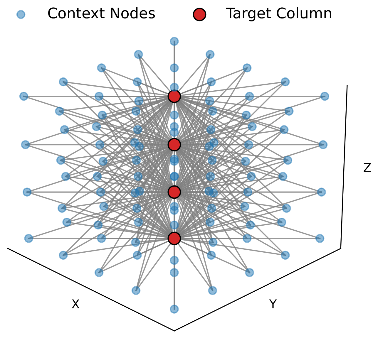
A graph network learns the iterative, non-local synthesis once and evaluates it cheaply thereafter: 10³× faster in 1D, 10⁶× in 3D. The graph is the paper's schematic of the one the 3D model works on: the populations are inferred in the target column (red) from the context points linked to it (blue). The model's own graphs have 11 × 11 × 55 nodes. ApJ 2022 · A&A 2026.
Generated in the browser from the same rules as the paper figure: ±2 neighbours, stride 1, radius 3.
From photons to inference

The pipeline I build, end to end

01 · Observephotons → counts
Telescope campaigns

PI on SST and GREGOR runs; calibration and reduction of spectropolarimetric data.

Python · IDL · pipelines
02 · Measurecounts → Stokes I,Q,U,V
Polarised spectra

Four Stokes profiles per pixel: the raw signal that encodes the magnetic field.

numpy
03 · Modelatmosphere → spectra
Non-LTE radiative transfer

Iterative, non-local forward model. Slow — which is the problem to solve.

C++ · MPI
04 · Learngraph → spectra, fast
GNN surrogate

A graph network learns stage 3 once, then evaluates it 10³× faster in 1D and 10⁶× in 3D.

PyTorch · PyG · GPUs
05 · Inferspectra → B-field + σ
3D inversion

Global minimisation over 3D geometry; error bars, no 180° ambiguity.

POLARIS · global optimisation

Every stage is one I have written code for — from telescope calibration scripts to the GPU-trained surrogate that replaces stage 3.

Timeline

2014 → today, hover to read

20142017202020232026
2014 – 2018 BSc in Physics Universitat de València Plus a research grant on mass estimation of galaxy clusters and an observatory internship at Aras de los Olmos.
Why industry, why now

The problems I like are the ones where the model is expensive and the data is messy.

That describes a solar prominence. It also describes demand forecasting, sensor fusion, risk models and simulation-based inference. Ten years of squeezing physical answers out of imperfect measurements — with error bars — is the part I want to keep. The subject can change.

Get in touch ORCID Sentiment Prism (side project) UpValuations (archived demo)
Skill map
Inference Deep learning HPC / MPI Software eng. Data pipelines Communication
Self-assessed
Compute
14.5MCPU-hours, 2019 – 2026
7.5M
La Palma supercomputer (RES, open access)
5M
MareNostrum, BSC (RES allocation)
2M
HLRS, Stuttgart (allocation as PI)
Stack
import numpy, scipy, matplotlib as daily_bread
from gnn_surrogates import torch, torch_geometric
from fine_tuning import transformers, wandb
from hpc import cpp, cuda, mpi, ssh
import slurm, git, docker, django, nginx

© 2026 Andrés Vicente Arévalo · Freiburg, Germany

 
  • ORCID

  • GitHub

  • [email protected]